Pipe Friction Loss Calculation: Darcy-Weisbach Formula, Reynolds Numbers & Moody Chart
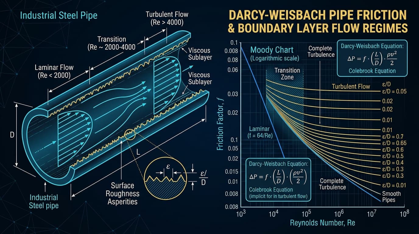
Figure 1: Boundary layer velocity distribution, viscous sublayer submergence, surface roughness asperities (ε), and Moody diagram friction factor curves.
The Foundation of All Hydraulic Calculations
Every pump sizing datasheet, pipeline surge analysis, and cooling circuit relies on calculating frictional head loss. While civil water engineers often use Hazen-Williams, industrial mechanical engineers must use the Darcy-Weisbach formulation to accurately account for fluid viscosity, temperature changes, and non-Newtonian flow regimes.
1. Why Empirical Formulas (Hazen-Williams) Fail in Real Plants
Many introductory textbooks still teach the Hazen-Williams empirical formula. However, Hazen-Williams has three catastrophic limitations:
- It was calibrated exclusively for ambient water at 15°C to 20°C (60°F). It cannot handle hot feedwater, thermal oil, hydrocarbons, or glycol solutions.
- It assumes friction is completely independent of viscosity and Reynolds number.
- It introduces sizing errors of up to 30% to 40% when operating outside room temperature!
By contrast, the Darcy-Weisbach equation is dimensionally homogeneous, theoretically rigorous, and valid for any liquid or gas across laminar, transitional, and fully turbulent flow regimes.
Automate Colebrook-White Friction Factors
Solve iterative pipe friction factors and velocity profiles dynamically using Zylofy's built-in fluid mechanics engine.
2. The Darcy-Weisbach Master Equation
Frictional head loss (h_f) in meters of fluid column is expressed as:
Where:
- f: Darcy friction factor (dimensionless)
- L: Length of pipe (meters or ft)
- D: Pipe internal diameter (meters or ft)
- v: Mean flow velocity (v = 4Q / (π D²)) [m/s or ft/s]
- g: Gravitational acceleration (9.80665 m/s² or 32.174 ft/s²)
- ρ: Fluid density at operating temperature (kg/m³)
3. Flow Regimes: Laminar, Critical Transition & Turbulent
To determine the friction factor (f), you must first evaluate the Reynolds number (Re):
Streamline parallel layers without mixing. Friction factor is independent of pipe roughness and depends solely on viscous shear: f = 64 / Re.
Unstable boundary layer where flow fluctuates unpredictably between laminar and turbulent. Engineers design piping velocities to avoid operating within this zone.
Violent micro-vortices and rapid momentum mixing. Friction factor depends on both Reynolds number and relative roughness (ε / D), solved via the Colebrook equation.
4. Solving for Friction Factor (f): Colebrook vs. Swamee-Jain
In turbulent flow, the friction factor is defined by the famous implicit Colebrook-White equation (1939):
Notice that √(f) appears on both sides of the equation! In modern software like Zylofy, this is solved via Newton-Raphson numerical iteration in 3 to 5 steps. For manual spreadsheet calculations, you can use the highly accurate explicit Swamee-Jain formula (error under 1% for 10⁻⁶ ≤ ε/D ≤ 10⁻² and 5000 ≤ Re ≤ 10⁸):
5. Pipe Surface Roughness (ε) Table for Industrial Materials
Surface roughness (ε) represents the average height of microscopic surface asperities on the pipe wall:
| Pipe Material | Roughness (ε) [mm] | Roughness (ε) [inches] | Design Notes |
|---|---|---|---|
| Commercial Carbon Steel (New) | 0.045 | 0.0018 | Standard seamless ASTM A106 / A53 |
| Carbon Steel (Aged / Light Rust) | 0.150 | 0.0059 | Use for 5+ year aged water piping |
| Stainless Steel (304 / 316) | 0.015 | 0.0006 | Smooth drawn industrial tubing |
| PVC, CPVC, HDPE & Fiberglass | 0.0015 – 0.005 | 0.0001 | Hydraulically smooth (no scale accumulation) |
| Ductile Iron (Cement Mortar Lined) | 0.030 | 0.0012 | Municipal water mains |
6. Minor Fitting Losses: Equivalent Length (L/D) vs. K-Factor
Turbulence around elbows, tees, reducers, and valves causes localized pressure drops called "minor losses" (which can easily exceed straight pipe losses in tight plant skids!):
Alternatively, using the Crane Technical Paper 410 method, you can express each fitting as an equivalent straight pipe length: L_eq = (L/D) · D. Summing L_straight + Σ L_eq allows you to calculate the entire pipe network with a single Darcy-Weisbach evaluation!
7. Full Worked Engineering Calculation: Sizing a 150m Cooling Line
Design Conditions:
- Flow Rate (Q): 120 m³/h (0.0333 m^3/s)
- Fluid: Water at 25°C (ρ = 997 kg/m³, ν = 0.893 × 10⁻⁶ m^2/s)
- Pipe: DN150 (6-inch Sch 40 Carbon Steel, Internal Diameter D = 154.1 mm = 0.1541 m)
- Pipe Length (L): 150 meters straight pipe
- Fittings: 6x 90° LR elbows (K = 0.3), 2x gate valves (K = 0.15), 1x check valve (K = 2.0)
- Pipe Roughness (ε): 0.045 mm
v = Q / A = 0.0333 / [ π · (0.1541/2)² ] = 1.788 m/s (Ideal industrial velocity)
Re = (1.788 · 0.1541) / (0.893 × 10⁻⁶) = 308,545 (Fully Turbulent)
ε / D = 0.045 / 154.1 = 0.000292
Solving Colebrook equation yields: f = 0.0168
h_f,pipe = 0.0168 · (150 / 0.1541) · [ 1.788² / (2 · 9.81) ] = 0.0168 · 973.4 · 0.1629 = 2.66 meters
ΣK = (6 · 0.30) + (2 · 0.15) + (1 · 2.00) = 1.8 + 0.3 + 2.0 = 4.10
h_minor = 4.10 · 0.1629 = 0.67 meters
h_f,total = 2.66 m + 0.67 m = 3.33 meters of head (0.325 bar pressure drop)
8. 4 Common Pipe Friction Sizing Pitfalls
Using Nominal Pipe Size (NPS) Instead of Actual Internal Diameter
A 6-inch pipe is not 6.000 inches ID. A Schedule 40 6-inch pipe is 6.065 inches ID, while a Schedule 80 6-inch pipe is 5.761 inches ID. Because diameter is raised to the 5th power in friction calculations, that small wall thickness difference increases head loss by over 28%!
Designing with Excessive Fluid Velocity to Save Pipe Cost
Running liquid above 3.0 m/s (10 ft/s) drastically increases friction loss and triggers acoustic pipe erosion and hydraulic water hammer.
Neglecting Viscosity Changes Across Temperature Swings
Heavy fuel oil or thermal fluid at 20°C can be 50 times more viscous than at 80°C. Sizing only for the hot design temperature will cause cold morning motor overloads.
Placing Elbows Immediately Upstream of Pump Suction
An elbow installed closer than 5 pipe diameters from the suction flange creates uneven flow velocity profiles entering the impeller eye, triggering localized cavitation.
9. Frequently Asked Questions
Does pipe wall roughness affect laminar flow friction?
No! In laminar flow (Re < 2300), fluid flows smoothly in parallel concentric layers. The fluid touching the wall is stationary (no-slip condition), and internal viscous friction occurs between fluid layers, completely submerging wall asperities. Roughness has zero effect on laminar friction factor (f = 64/Re).
What is a good rule of thumb for liquid piping velocity?
For pump suction lines: 0.8 to 1.5 m/s (2.5 to 5.0 ft/s) to preserve suction pressure and prevent cavitation. For pump discharge lines: 1.5 to 2.5 m/s (5.0 to 8.0 ft/s) to balance capital pipe cost against ongoing pumping energy consumption.
Zylofy Thermal & Fluid Dynamics Engineering Group
Authored and reviewed by computational hydraulics engineers and piping stress specialists with expertise in industrial fluid modeling, Colebrook-White solvers, and power plant pipe sizing.